5. Group assignment: Analysis of flow past backward
facing step by using k-omega SST turbulence model
The project is aimed at the
investigation of flow pattern past a backward facing step of variable (a) top wall angle. Results are to be compared
with experimental data.
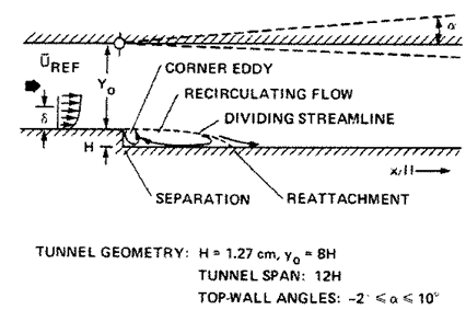
Figure 1. Geometrical model and flow structures.
The backward facing step is located at
the lower wall of a channel. The channel has an even width in the direction
perpendicular to the x-y plane, that is, a two-dimensional flow can be assumed.
The channel height is Y0(=8H)
on the upstream side and Y0+H
on the downstream side of the step; the step height is H. Since each dimension can be expressed in terms of H, only H=12.7mm is specified. The origin of
the coordinate system (x=0, y=0) is specified by the upper corner of the step,
the inlet is located at x=-2H. The
outlet cross-section is at 15H away
from the step. The upper wall can be tilted about a turning point just above
the step. In this way, the channel can shrink or expand in steamwise direction
creating a positive or negative pressure gradient. Angle a is measured between the upper (tilted)
wall and the initial flow direction.
Boundary
conditions
Velocity and turbulence characteristics
are imposed at the inlet boundary according to bfs_belepes.prof.
It is important to note, that inlet quantities are specified at x=-2H (upstream
from the step), therefore the geometrical model need to be prepared
correspondingly. Turbulent kinetic energy (k), turbulent dissipation rate
(epsilon) and specific dissipation rate (omega) are contained by the profile
file. Use pressure boundary condition at the outlet, and no-slip condition on
solid walls.
The reference velocity used in the
evaluation of dimensionless quantities is Uref=44.2m/s
. Note that, this is not a boundary condition!
Task 1. (3 points)
Preparation of the geometrical model
with alfa=-2°, 0°, 6° and 10°;
Generation of block structured mesh;
Please mind that:
- the boundary layers on solid walls,
require a proper wall-normal resolution;
- and the shear layer, separated from
the upper edge of the step, also needs refinements.
Task 2. (3 points)
Selection and parameterization of
boundary condition in FLUENT;
Use the given inlet profile for
specifying inlet boundary conditions!
Task 3. (3 points)
Check your mesh for meeting turbulence
model criteria as well as resolution required at highly sheared zones for alfa=0
lid angle:
- check if the value of y+ is within the
range required by the turbulence model; if not, modify your mesh accordingly;
- perform adaptive refinement in the
vicinity of the shear layer and evaluate changes in flow characteristics.
Task 4. (3 points)
Run simulations with k-omega SST
turbulence model for 4 different alfa angle!
- Plot velocity profiles downstream from
the step in 1H, 2H, 3H and 4H distances!
- Compare the calculated reattachment
lengths resulted with measured values (xR/H)!
- Compare the calculated pressure
coefficient (cp) profiles, with special attention to the correct
selection of reference values.
Measured data:
Position of the reattachment point
|
Lid angle |
Reattachment length |
Error |
|
a [°] |
Xr/H |
dXr/H |
|
-2 |
5.82 |
-0.08 |
|
0 |
6.26 |
-0.1 |
|
6 |
8.3 |
-0.15 |
|
10 |
10.18 |
-0.5 |
Pressure coefficient (cp) on lower wall (on the side of the step)
|
X/H |
a=-2 |
a=0 |
a=6 |
a=10 |
|
-8.5 |
0 |
0.0039 |
0.0117 |
0.0088 |
|
-6.5 |
0 |
0 |
0.0136 |
0.0108 |
|
-4.5 |
-0.0059 |
-0.0048 |
0.0166 |
0.0187 |
|
-2.5 |
-0.0296 |
-0.0231 |
0.0214 |
0.0266 |
|
-0.5 |
-0.0642 |
-0.0472 |
0.0283 |
0.0512 |
|
0 |
-0.0859 |
-0.0607 |
0.0361 |
0.061 |
|
0.5 |
-0.0899 |
-0.0636 |
0.0331 |
0.06 |
|
1 |
-0.0899 |
-0.0665 |
0.0312 |
0.0571 |
|
1.5 |
|
|
0.0292 |
0.0571 |
|
2 |
-0.1017 |
-0.0742 |
0.0253 |
0.0571 |
|
2.5 |
|
|
|
0.0502 |
|
3 |
-0.1037 |
-0.0762 |
0.0185 |
0.0482 |
|
3.5 |
-0.083 |
-0.0665 |
0.0253 |
|
|
4 |
-0.0464 |
-0.0424 |
0.04 |
0.0581 |
|
4.5 |
0.0049 |
0.0077 |
0.0585 |
|
|
5 |
0.0494 |
0.0482 |
0.0829 |
0.0876 |
|
5.5 |
0.0771 |
0.0782 |
|
|
|
6 |
0.1037 |
0.1129 |
0.1297 |
0.1251 |
|
6.5 |
0.1205 |
0.1303 |
|
|
|
7 |
0.1275 |
0.1389 |
0.1667 |
0.1556 |
|
8 |
0.1304 |
0.1515 |
0.1989 |
0.1871 |
|
8.5 |
|
|
0.2115 |
|
|
9 |
0.1225 |
0.1535 |
0.2203 |
0.2117 |
|
9.5 |
|
|
0.231 |
|
|
11 |
0.0978 |
0.1477 |
0.2544 |
0.2551 |
|
12 |
|
|
0.2641 |
|
|
13 |
0.0751 |
0.1409 |
0.2749 |
0.2846 |
|
15 |
0.0534 |
0.1342 |
0.2924 |
0.3073 |
|
17 |
0.0385 |
0.1303 |
0.308 |
0.328 |
|
19.5 |
0.0168 |
0.1285 |
0.3265 |
0.3448 |
|
21.5 |
0.001 |
0.1246 |
0.3402 |
0.3596 |
|
23.5 |
-0.0168 |
0.1227 |
0.3528 |
0.3723 |
|
25.5 |
-0.0346 |
0.1227 |
0.3674 |
0.3813 |
|
27.5 |
-0.0494 |
0.1218 |
0.3821 |
0.3921 |
|
29.5 |
-0.0652 |
0.1218 |
0.3889 |
0.4011 |
|
31.5 |
-0.085 |
0.1199 |
0.4035 |
0.409 |
|
33.5 |
-0.1048 |
0.116 |
0.4133 |
0.4139 |
|
35.5 |
-0.1236 |
0.1189 |
0.4279 |
0.4198 |
|
37.5 |
-0.1463 |
0.1141 |
0.4347 |
0.4209 |
Pressure coefficient (cp) on upper wall (opposite to the step)
|
X/H |
a=-2 |
a=0 |
a=6 |
a=10 |
|
-5 |
0.0178 |
0.0087 |
0.0039 |
-0.0108 |
|
3 |
0.0306 |
0.0414 |
0.0799 |
0.0896 |
|
5 |
0.03 |
0.0511 |
0.1248 |
0.1536 |
|
7 |
0.0296 |
0.0598 |
0.1627 |
0.1989 |
|
9 |
0.0425 |
0.081 |
0.1989 |
0.2471 |
|
11 |
0.0504 |
0.0993 |
0.232 |
0.2816 |
|
13 |
0.0454 |
0.1118 |
0.2612 |
0.3092 |
|
15 |
0.0336 |
0.1138 |
0.2846 |
0.3338 |
|
17 |
0.0286 |
0.1206 |
0.308 |
0.3545 |
|
19 |
0.0148 |
0.1216 |
0.3246 |
0.3683 |
|
21 |
0.001 |
0.1216 |
0.3402 |
0.3821 |
|
23 |
-0.0158 |
0.1207 |
0.3538 |
0.389 |
|
25 |
-0.0296 |
0.1236 |
0.3713 |
0.3979 |
|
27 |
-0.0474 |
0.1217 |
0.384 |
0.4029 |
|
29 |
-0.0642 |
0.1208 |
0.3947 |
0.4079 |
|
31 |
-0.0811 |
0.1189 |
0.4055 |
0.4178 |
|
33 |
-0.1038 |
0.116 |
0.4133 |
0.4178 |
|
35 |
-0.1236 |
0.1179 |
0.4298 |
0.4228 |
|
37 |
-0.1464 |
0.1131 |
0.4396 |
0.4239 |
Task 5. (3 points)
Plot the streamlines colored by velocity
magnitude, the static and total pressures as well as the turbulent kinetic energy
and save images in TIF format.
Briefly describe the investigation aims,
the solution methods, and the results in comparison to measurement data.
Prepare your report in PowerPoint (.PPT) format and
upload to the folder specified by the practice leader!